Statistics
Scales
- nominal (categorical without order): A blue, B red, C green … (no meaningful relation between the numbers)
- rank (categorical with order): A junior, B middle, C senior, D principal … (B > A)
- intervals (numerical without natural zero): A $10^\circ$, B $20^\circ$, C $30^\circ$ … (B > A, B-A = D-C), allows +/- operations.
- ratio (numerical with natural zero): A 10km., B 20km. C 30km. (B > A, B is twice faster than A), allows +/- and */div operations
Descriptions
- dispersion and shape is the extent to which a distribution is stretched and squeezed
- mean where population mean is $\mu$ and sample mean $\overline {x}$, calculated the same way.
- variance: $\displaystyle {Var} (X)=\frac {1}{n} \sum _{i=1}^n (x_i - \mu )^2 = \sum _{i=1}^n p_i \times (x_i - \mu )^2$
- for continuous var $\displaystyle \int \mathrm{d}x \ p(x) \ (x-\mu)^2$, where $f(x)$ is the PDF
- for sample variance use $1/(n-1)$ instead of $1/n$, where the $-1$ is to compensatione for sample varaince being always samller than population varaince.
- co-variance classify positive, negative and no relationship. But tells nothing about the slope itself (i.e. different values could show the same correlation).
- sample SD = $\sqrt {varaince} = \displaystyle \sqrt \frac {\sum _{i=1}^n (x_i - \overline x)^2}{n-1}$. In the general case we use the “sample” varaince and SD, not the population one (i.e divide by $n-1$ instead of $n$).
- inter-quartile range $Q_{3}-Q_{1}$ or $75^{th}$ and $25^{th}$ percentiles.
- coefficient of variation (or relative SD) = $\displaystyle {\frac {\sigma }{\mu }}$
- $standard\ error = sample\ SD/\sqrt{sample\ N}$
- Moments
Means
Pythagorean
- arithmetic - good for data with linear relationship $\displaystyle \frac {1}{n} \sum _{i=1}^n a_i = \frac {a_1 + a_2 + \cdots +a_n}{n}$
- $\mu = E[x] = \sum_x p(x)x = \int \mathrm{d}x \ p(x)x$, where $E[x]$ is expected value
- geometric - good for data with multiplicative relationship : $\displaystyle \left(\prod _{i=1}^n a_i \right)^{\frac 1 n} = \sqrt[n] {(a_1 \times a_2 \times \cdots \times a_n)}$
- Data is of different scales, but then we no longer have an interpretative scale. Geometrical mean is unit-less.
- The above formulae cannot accommodate with inputs $\leq 0$, due to the multiplication part.
-
- useful when comparing items with different ranges (e.g. $a_1$ is from 0 to 1 and $a_2$ is from 0 to 100).
- harmonic - good for ratios $[(i_1^{-1} + i_{…}^{-1} + i_n^{-1})/n]^{-1}$, that is to say the the harmonic mean is the reciprocal of the arithmetic mean of reciprocals.
- The above formulae cannot accommodate with inputs $\leq 0$, due to the division part.
- remember from primary school that the reciprocal of $n$ is $1/n$, and for $y/x$ it is $x/y$ (i.e. $1 - y/x = x/y$). Anther way to think of reciprocal is about two numbers that equal 1 when multiplied together.
- $5 \div 3/7 = 5/1 * 7/3 = 35/3$
- Example: trip from $A$ to $B$ and back: $A\to B\ 30\ km/h$, $B\to A\ 10\ km/h$
- Solution with arithmetic mean requires to use the time spent:
- $A\to B\ : 30\ km\ per\ 60\ min => 1/2\ km\ per\ min => 5\ km\ at\ 1/2\ speed = 10\ mins$
- $B\to A\ : 10\ km\ per\ 60\ min => 1/6\ km\ per\ min => 5\ km\ at\ 1/6\ speed = 30\ mins$
- Total time = $10 + 30 = 40\ mins$, so $A\to B$ accounts for $25\%$ of the total time and $B\to A$ accounts for $75\%$ of total time.
- Weighted arithmetic mean = $(30\ km/h * 0.25) + (10\ km/h * 0.75) = 15km/h$
- Solution with harmonic mean:
- arithmetic mean of reciprocals = $1/30 + 1/10 = (2/15) / 2 = 1/15$
- reciprocal of the arithmetic mean = $1 \div 1/15 = 1/1 * 15/1 = 15$
- (another way of typing it) : $\displaystyle \frac {n}{\sum \limits _{i=1}^n \frac {1}{x_i}} = \frac {n}{\frac {1}{x_1} + \frac {1}{x_2} +\cdots + \frac {1}{x_n}}$
- useful for situations when the average of rates is desired.
Descriptive
- median
- mode
- skewness
- kurtosis
Generalized
With specific distributions
With specific geometries
- Freshet mean
Null hypothesis:
- Elementary statistial inference does not “accept” nor “confirm”.
- Reject the null hypothesis.
- Fail to reject the null hypothesis.
Errors and residuals // when comparing to a value
- error is the deviation of the observed value from the true value (the population mean).
- $e_i = X_i - \mu$
- The expected value, being the mean of the entire population, is typically unobservable, and hence the statistical error cannot be observed either.
- $e_i = X_i - \mu$
- residual (fitting deviation) is the deviation of the observed value from the estimated value (the sample mean).
- $e_r = X_r - \bar {X}$
- BIASES and other uses:
- SSE (sum of square errors or residuals) refers to the residual sum of squares (SSR) of a regression.
- MSE and RMSE refer to the amount by which the values predicted by an estimator differ from the quantities being estimated
Moments
- TODO: ++ https://en.wikipedia.org/wiki/Moment_(mathematics)
- https://en.wikipedia.org/wiki/Standardized_moment
- https://en.wikipedia.org/wiki/L-moment
- https://www.itl.nist.gov/div898/software/dataplot/refman2/auxillar/lmoment.htm
- The primary use of probability weighted moments and L-moments is in the estimation of parameters for a probability distribution. Estimates based on probability weighted moments and L-moments are generally superior to standard moment-based estimates. The L-moment estimators have some desirable properties for parameter estimation. In particular, they are robust with respect to outliers and their small sample bias tends to be small. L-moment estimators can often be used when the maximum likelihood estimates are unavailable, difficult to compute, or have undesirable properties. They may also be used as starting values for maximum likelihood estimates.
PDFs
- Probabilities are the areas under a fixed curve $p(data \mid distribution)$
- Likelihoods are the y-axis values for a fixed point with distributions that can be moved $L(distribution \mid data)$
- TODO: ++ https://en.wikipedia.org/wiki/Kernel_density_estimation
Power and Sample Size
- Power is the probability that we will corectly reject the null hypothesis (e.g. correctly get a small $p$ value). Commonly denoted as $1 - \beta$ (a.k.a. true positive), where $\beta$ is the probability of type II error (a.k.a. false negative).
- $\alpha$ is the probability of false positive, and $1 - \alpha$ us true negative
- To do a power calculation, one needs 2 out of 3 : effect szie, data variation and sample size.
- If there are is a preliminary data use it for effect size and data variation.
- if no preliminary data is available: do 3 replicas, look for a 2 fold difference and see how much variation will gice a good power. If vraintion is small increase sample size or effect size.
- for some fata there is already calculated variantion. So either plugin the wanted effect size and determine the sample size, or vice-versa.
- A simple way for power calculaton:
- choose a good power between 0 and 1, often 0.8 (e.g. 80% of correctly rejecting the null hypothesis)
- choose a good significance threshold $\alpha$ e.g 0.05
- calculate effect size $d$
- online calculators
- Power and Sample Size
- Power and Sample Size - Main Menu
- Power of a test (wiki) and Predictive probability of success (wiki)
Survival function / analysis
- In the general case the survival function = 1 - CDF.
Scaling and Normalizing
- In scaling the range of the distributed data is changed, but shape and property stays the same (i.e. fit data between min-max range).
- simple scaling $X_{new} = X_{old} / X_{max}$
- min max scaling $X_{new} = (X_{old}-X_{min}) / (X_{max}-X_{min})$
- In normalizing the shape of the distributed data is changed.
- In the general case it is transformed to normal distribution.
- referred also as Standardization.
- Z score - how far away is an item from the mean.
- Box-Cox normalization
- T-Scores…
Expected value
-
probability 0.17 0.83 outcome -1 1 - Expected values is the sum of each outcome $x$ times the probability of observing it $P(X=x)$. \(E(X) = (-1 \times 0.17)+(1 \times 0.83) = 0.66 = \sum x\ P(X=x)\)
- (with exponential distribution below) Probability of meeting someone.
- Meet someone in 10 secondes, then calculate the AUC between 0 and 10 is $\displaystyle \int_0^{10} \lambda e^{-\lambda x} = 0.39$ or between 25 and 30 seconds $\displaystyle \int_{25}^{30} \lambda e^{-\lambda x}$
- Note: total AUC is 1.
- Alternatively, the probabilitu of meeting someone in the first 10 seconds is approximately the width of the rectangle 0 to 10, which is $(10-0)=10$ times its height.
- to find the height, find the y-xais coordinate where the top edge of the reactange intersects the curve (e.g. when time = 5) : $f(X=5, \lambda=0.05)= \lambda e^{-\lambda x} = 0.05 e^{-0.05 \times 5} = 0.04$.
- meeting someone between 0 and 10 secs = Area = hieght * width = $0.04 \times 10 = 0.04$, compared to $0.39$ calculated above.
- Then do this for each 10 seconds interval.
- Then put these into the equation for discrete outcomes, to get how much, on average, one must wait to meet someone. Let’s say the result is 22.
- Then do these for 5 second intervals (rectangles will double). Let’s say the result is 21.8.
- Then go for 0 second interval an infinite number of rectangles, then we are not approximationg, but calculating exactly.
- So the height at each point is the likelihood at that point and the width can be written as $\Delta x$ And when the number of rectangles $n$ goes to $\infty$, than $\Delta x$ goes to $0$ one ends up with an integral.
\(\lim_{n \rightarrow \infty} E(X) = \sum_{i=1}^{n=\infty} x\ P(X=x) =\) \(= \sum_{i=1}^{n=\infty} width \times height = \lim_{n \rightarrow \infty} \sum x\ (L(X=x) \times \Delta x) =\) \(=\int x\ L(X=x) dx\)
- So for calculation the Expected value thru an exponential distribution $f(X=x) = \lambda e^{-\lambda x}$, just plug it in the formula above. Just have in minf that the exponential formula is define for values greater than $0$. This will give us 20 seconds: \(E(X) = \int_0^{\infty} x\ \lambda e^{-\lambda x}\ dx\)
example of exponential distribution
- $f(X=x)= \lambda e^{-\lambda x}$, when $x \geq 0$, otherwise $0$. In the example below $\lambda$, which is also called the Rate, is a parameter that defines the shape of the curve. Examples with $\color {azure} {\lambda = 0.05}$ and $\color {orange} {\lambda = 0.01}$
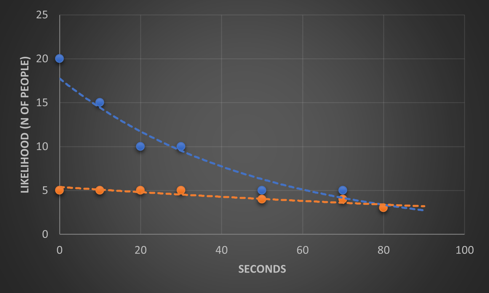 ){:height=”50%” width=”50%”}
Some nice examples
- Odds Ratios and Logs Example for Determine the p-value of the significance of relationship. Check the same example with Bayesian too, might be a fun!!!
- PCA compare correlations. PCoordinateA compares distances. Note: mnimizing Euclidean (linear) distances is the same as maximizing Euclidean (linear) correlations (PCA).
- MDS (multi-dimensional scaling) uses log fold change
- there are many other distances however
- for eigen stuff see StatQuest - PCA
References
- Starmer, J. StatQuest! https://statquest.org/